Handling and Plotting data in Octave / MATLAB

What's in memory

To quickly view the variables in memory, use the who command. Use whos for detailed view

>> who
Variables in the current scope:
ans       ar1       heat      readings  vec       vec1      vec44     vec45     x         y         z

>> whos
Variables in the current scope:
   Attr Name          Size                     Bytes  Class
   ==== ====          ====                     =====  =====
        ans           1x78                        78  char
        ar1           1x4                         32  double
        heat          1x1                          8  double
        readings      4x4                        128  double
        vec           1x16                        24  double
        vec1          1x4                         32  double
        vec44         4x4                        128  double
        vec45         4x5                        160  double
        x             1x21                        24  double
        y             1x21                       168  double
        z             1x21                       168  double

Total is 218 elements using 950 bytes

To delete a variable from memory, use the clear <variable name> command. Just using the clear command will remove all variables.

Reading data files

Read datasets with load command. >> load('ex1data1.txt') A variable with the name of the file is created in memory. You can use array slicing, dicing to move a part of this data into a new variable.

>> load('ex1data1.txt');
>> subset = ex1data1(1:10,:)
subset =
    6.1101   17.5920
    5.5277    9.1302
    8.5186   13.6620
    7.0032   11.8540
    5.8598    6.8233
    8.3829   11.8860
    7.4764    4.3483
    8.5781   12.0000
    6.4862    6.5987
    5.0546    3.8166

Saving data to disk

Use save <filename.extn> <variable> <-options> to save a variable to disk.

>> save 'subset.mat' subset

You can load this back into memory using the load command: load('subset.mat'). This time, since it is a mat file, Octave will load it with the original variable name.

To save data in a human readable form, use save <filename.txt> <variable> -ascii.

Plotting

Most 2D plots can be accomplished using plot(<arr1>, <arr2>, 'srt:options') function.

Line plots

plot(x,y); % will plot in a new window

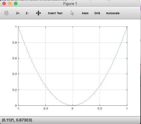
We can customize the appearance of ticks and line by passing them as a string. For instance, r:* will make lines in red, * for points and : for dotted lines.

You can also customize the title, labels, legend as shown:

>> plot(x,y);
>> xlabel('time[x]');
>> ylabel('y=x^2');
>> legend('y(x)')
>> title('Function of time')

Overlaying plots

To overlay multiple plots on the same frame, use hold on command.

>> z = x.^3;
>> plot(x,y, 'r:o')
>> hold on
>> plot(x,z, 'g--*')

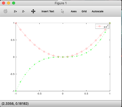
You can also plot multiple plots in the same command as plot(x,y, x,z) which will overlay both y and z on the same plot window.

To close the current figure, call the close command.

Printing plots to disk

To print to disk, use the print command as print -dpng 'myplot.png'. This will print the current plot to disk.

Multiple plot windows

Use the figure(n) command to create new plot windows:

>> figure(1); plot(x,y1);
>> figure(2); plot(y1,y2);

will open 2 plot windows, one for each plot command.

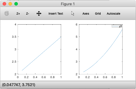
Subplots

Use the subplot(nrows, ncols, current_cell) command to create and activate a plot window:

>> subplot(1,2,1);
>> plot(x,y1);
>> axis([0,1]);  % Sets axis limits. Syntax is axis([xmin, xmax, ymin, ymax])
>> subplot(1,2,2);
>> plot(x,y2);
>> legend('y2');

which produces:

Visualizing matrices as images

To quickly 'see' a matrix as a color coded image, use imagesc:

>> x=randn(900,1);  % produces a standard normal dist, mean=0
>> size(x)
ans =
   900     1
>> x2d= reshape(x,30,30); % turns this vector to a 2d matrix
>> imagesc(x2d);  % turns this matrix to an image
>> colorbar;  % adds a colorbar legend