Analytical vs Gradient Descent methods of solving linear regression
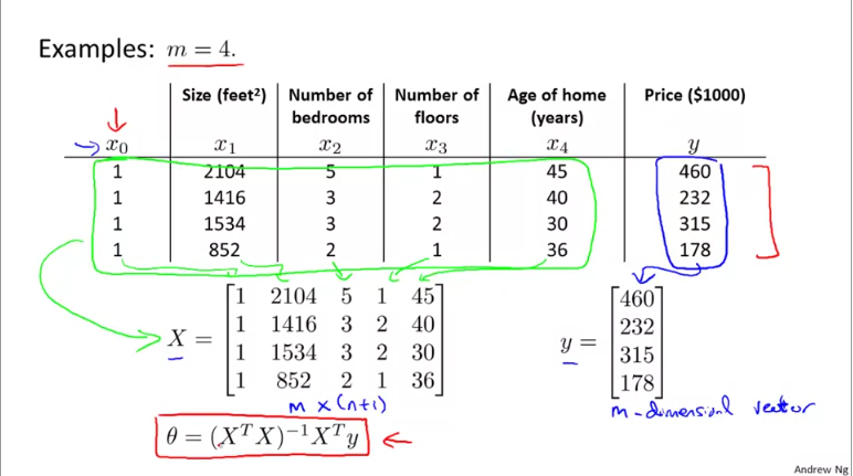
The Gradient Descent offers an iterative method to solve linear models. However, there is a traditional and direct way of solving it called as normal equations. In normal equations, you build a matrix where each record of observation becomes a row (m rows) and each feature becomes a column. You prefix an additional column to represent the constant (n+1 columns). This matrix, represented as X is of dimension m x (n+1). You represent the response variable as a vector y of dimension m x 1.

The formula to calculate the optimal coefficients is given by \(\theta = (X^{T}X)^{-1}X^{T}y\). Where \(\theta\) is a vector of shape n+1 containing \([\theta_{0}, \theta_{1} ... \theta_{n}]\).
Caveats when applying analytical technique
- In the analytical, normal equation method, there is no iteration to arrive at optimal \(\theta\). You simply calculate it.
- You do not have to scale features. It is ok to have them in their native dimensions.
Guidelines for choosing between GD and Normal equation
- GD needs you to play with \(\alpha\) (learning rate), while normal equation does not.
- GD is an iterative process, while normal eq is not.
- GD shines well when you have a large number of attributes / features / independent variables. The order of GD is given by \(O(kn^{2})\) for
nfeatures. - Normal equation needs to invert a matrix which is an expensive operation. Its time complexity is given by \(O(n^{3})\).
- If you have
>10,000independent variables, or if the number of observations / rows is less than number of independent variables (m < (n+1)), then normal equation not produce a matrix that is invertible. You are better off with Gradient Descent regression. - If you have highly correlated features (multi-collinearity) or when you have more features than observations, you might end up with a non-invertible matrix for the normal equation. In these cases, you can choose GD or you can delete some features or regularization techniques if you want to continue with normal equation.
- GD is an approximation technique, while normal equation is a deterministic approach. GD might settle in a local minima and not global minima. Although, for linear regressions, the shape of the loss function is such that there is no local but only a global minima.