Implementing Gradient Descent for Linear Regression
For a theoretical understanding of Gradient Descent visit here. This page walks you through implementing gradient descent for a simple linear regression. Later, we also simulate a number of parameters, solve using GD and visualize the results in a 3D mesh to understand this process better.
Load the data
import pandas as pd
import plotly_express as px
import numpy as np
import matplotlib.pyplot as plt
import os
from mpl_toolkits import mplot3d

from plotly.offline import download_plotlyjs, init_notebook_mode
from plotly.offline import plot, iplot
#set notebook mode
init_notebook_mode(connected=True)
path='/Users/atma6951/Documents/code/pychakras/pyChakras/ml/coursera-ml-matlabonline/machine-learning-ex/ex1'
data_df = pd.read_csv(os.path.join(path, 'ex1data1.txt'), header=None, names=['X','y'])
data_df.head()
| X | y | |
|---|---|---|
| 0 | 6.1101 | 17.5920 |
| 1 | 5.5277 | 9.1302 |
| 2 | 8.5186 | 13.6620 |
| 3 | 7.0032 | 11.8540 |
| 4 | 5.8598 | 6.8233 |
data_df.shape
(97, 2)
n_rows = data_df.shape[0]
X=data_df['X'].to_numpy().reshape(n_rows,1)
# Represent x_0 as a vector of 1s for vector computation
ones = np.ones((n_rows,1))
X = np.concatenate((ones, X), axis=1)
y=data_df['y'].to_numpy().reshape(n_rows,1)
X.shape, y.shape
((97, 2), (97, 1))
Plot the dataset
plt.scatter(x=data_df['X'], y=data_df['y'])
plt.xlabel('X'); plt.ylabel('y');
plt.title('Input dataset');
Create a cost function
Here we will compute the cost function and code that into a Python function. Cost function is given by
$$ J(\theta_{0}, \theta_{1}) = \frac{1}{2m} \sum_{i=1}^{m} (h_{\theta}(x_{i}) - y_{i})^2 $$
where $h_{\theta}(x_{i}) = \theta^{T}X$
def compute_cost(X, y, theta=np.array([[0],[0]])):
    """Given covariate matrix X, the prediction results y and coefficients theta
    compute the loss"""

    m = len(y)
    J=0 # initialize loss to zero

    # reshape theta
    theta=theta.reshape(2,1)

    # calculate the hypothesis - y_hat
    h_x = np.dot(X,theta)

    # subtract y from y_hat, square and sum
    error_term = sum((h_x - y)**2)

    # divide by twice the number of samples - standard practice.
    loss = error_term/(2*m)

    return loss
compute_cost(X,y)
array([32.07273388])
Solve using Gradient Descent
Using GD, we simultaneously solve for theta0 and theta1 using the formula: $$ repeat \; until \; convergence $$ $$ \theta_{0} := \theta_{0} - \alpha \frac{1}{m} \sum_{i=1}^{m} [(h_{\theta}(x_{i}) - y_{i})x^{(0)}_{i}] $$ $$ \theta_{1} := \theta_{1} - \alpha \frac{1}{m} \sum_{i=1}^{m} [(h_{theta}(x_{i}) - y_{i})x^{(1)}_{i}] $$
def gradient_descent(X, y, theta=np.array([[0],[0]]),
                    alpha=0.01, num_iterations=1500):
    """
    Solve for theta using Gradient Descent optimiztion technique.
    Alpha is the learning rate
    """
    m = len(y)
    J_history = []
    theta0_history = []
    theta1_history = []
    theta = theta.reshape(2,1)

    for i in range(num_iterations):
        error = (np.dot(X, theta) - y)

        term0 = (alpha/m) * sum(error* X[:,0].reshape(m,1))
        term1 = (alpha/m) * sum(error* X[:,1].reshape(m,1))

        # update theta
        term_vector = np.array([[term0],[term1]])
#         print(term_vector)
        theta = theta - term_vector.reshape(2,1)

        # store history values
        theta0_history.append(theta[0].tolist()[0])
        theta1_history.append(theta[1].tolist()[0])
        J_history.append(compute_cost(X,y,theta).tolist()[0])

    return (theta, J_history, theta0_history, theta1_history)
%%time
num_iterations=1500
theta_init=np.array([[1],[1]])
alpha=0.01
theta, J_history, theta0_history, theta1_history = gradient_descent(X,y, theta_init,
                                                                   alpha, num_iterations)
CPU times: user 247 ms, sys: 2.52 ms, total: 250 ms
Wall time: 248 ms
theta
array([[-3.57081935],
       [ 1.16038773]])
Plot Gradient Descent
We visualize the process of reducing the loss function using gradient descent in this graph
fig, ax1 = plt.subplots()

# plot thetas over time
color='tab:blue'
ax1.plot(theta0_history, label='$\\theta_{0}$', linestyle='--', color=color)
ax1.plot(theta1_history, label='$\\theta_{1}$', linestyle='-', color=color)
# ax1.legend()
ax1.set_xlabel('Iterations'); ax1.set_ylabel('$\\theta$', color=color);
ax1.tick_params(axis='y', labelcolor=color)

# plot loss function over time
color='tab:red'
ax2 = ax1.twinx()
ax2.plot(J_history, label='Loss function', color=color)
ax2.set_title('Values of $\\theta$ and $J(\\theta)$ over iterations')
ax2.set_ylabel('Loss: $J(\\theta)$', color=color)
ax1.tick_params(axis='y', labelcolor=color)

# ax2.legend();
fig.legend();
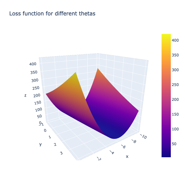
Compute cost surface for an array of input thetas
Let us synthesize a range of theta values and compute the cost surface as a mesh. We will then overlay the path our GD algorithm took to reach the optima
%%time
# theta range
theta0_vals = np.linspace(-10,0,100)
theta1_vals = np.linspace(-1,4,100)
J_vals = np.zeros((len(theta0_vals), len(theta1_vals)))

# compute cost for each combination of theta
c1=0; c2=0
for i in theta0_vals:
    for j in theta1_vals:
        t = np.array([i, j])
        J_vals[c1][c2] = compute_cost(X, y, t.transpose()).tolist()[0]
        c2=c2+1
    c1=c1+1
    c2=0 # reinitialize to 0
CPU times: user 566 ms, sys: 32.6 ms, total: 598 ms
Wall time: 569 ms
import plotly.graph_objects as go
fig = go.Figure(data=[go.Surface(x=theta0_vals, y=theta1_vals, z=J_vals)])
fig.update_layout(title='Loss function for different thetas', autosize=True,
                  width=600, height=600, xaxis_title='theta0',
                 yaxis_title='theta1')
fig.show()

num_iterations=1500
theta_init=np.array([[-5],[4]])
alpha=0.01
theta, J_history, theta0_history, theta1_history = gradient_descent(X,y, theta_init,
                                                                   alpha, num_iterations)
plt.contour(theta0_vals, theta1_vals, J_vals, levels = np.logspace(-2,3,100))
plt.xlabel('$\\theta_{0}$'); plt.ylabel("$\\theta_{1}$")
plt.title("Contour plot of loss function for different values of $\\theta$s");
plt.plot(theta0_history, theta1_history, 'r+');