A Primer on Linear Algebra

A mxn matrix is given by

\[ R^{mn} = \begin{bmatrix} a&b&c \\\ f&n&i \\\ c&b&w \end{bmatrix}_{3\times3} \]

where \(m\) is number of rows and \(n\) is number of columns.

A vector is a single column matrix and is given by

\[ v = \begin{bmatrix} a\\\ b\\\ d\\\ h\\\ j \end{bmatrix} \]

with \(5\) rows.

Notations

1. \(A_{ij}\) refers to element in \(i\)th row, \(j\)th column.
2. In general matrixes are 1 indexed - both in math and in Matlab
3. \(v_{i}\) refers to element in \(i\)th row of a vector
4. A vector with n rows is considered an n-dimensional vector
5. Matrices are denoted in uppercase and vectors and scalars in lower case.

Matrix operations

Matrix addition and subtraction

You cannot add a scalar to a matrix. You can however add two matrices, they need to be of same dimensions. You add each element at corresponding positions.

\[ \begin{bmatrix} 3&5\\\ 7&8\\\ -9&0 \end{bmatrix} + \begin{bmatrix} 8&0\\\ 5&-2\\\ 2&1 \end{bmatrix} = \begin{bmatrix} 3+8&5+0\\\ 7+5&8-2\\\ -9+2&0+1 \end{bmatrix} \]

The same applies for subtraction.

Matrix and scalar multiplication and division

You can multiply a scalar with a matrix, there are not restrictions with respect to dimensions. You multiply or divide each element with the same scalar.

\[ 3 \times \begin{bmatrix} 3&5\\\ 7&8\\\ 9&0 \end{bmatrix} = \begin{bmatrix} 9&15\\\ 21&24\\\ 27&0 \end{bmatrix} \]

Division is similar.

Matrix and vector multiplication

\[ \begin{bmatrix} a&b&c\\\ f&n&i\\\ c&b&w \end{bmatrix}^{\rightarrow}_{3\times3} \times \begin{bmatrix} 3\\\ 7\\\ 9 \end{bmatrix}\downarrow = \begin{bmatrix} 3a + 7b + 9c\\\ 3f + 7n + 9i\\\ 3c + 7b + 9w \end{bmatrix} \]

Solving linear equations as matrix operations

For optimization, you can represent linear equations as matrix operations. For instance, consider the hypothesis function \(h_{\theta}x = -40 + 0.45x_{i}\). To compute the hypothesis for \(n\) different values of \(x_{i}\) (34,56,21,11,10), you can represent the calculation as a matrix operation:

$$ \begin{bmatrix} 1& 34\\ 1& 56\\ 1& 21\\ 1& 11\\ 1& 10 \end{bmatrix} \times \begin{bmatrix} -40\\ 0.45 \end{bmatrix} = \begin{bmatrix} -24.7\\ -14.8\\ -30.55\\ -35.5\\ -35.5 \end{bmatrix} $$ Such matrix computation is way faster than a loop. This is applicable for most language including java, c++, octave, python.

Matrix x matrix multiplication

To multiply two matrices, the number of columns of first should match number of row of second => (mxn x nxp = mxp matrix).

\[ \begin{bmatrix} a&b&c\\\ f&n&i\\\ c&b&w \end{bmatrix} \times \begin{bmatrix} 3&1\\\ 7&2\\\ 9&3 \end{bmatrix} = \begin{bmatrix} (3a + 7b + 9c)&(1a + 2b+3c)\\\ (3f + 7n + 9i)&(1f+2n+3i)\\\ (3c + 7b + 9w)&(1c+2b+3w) \end{bmatrix} \]

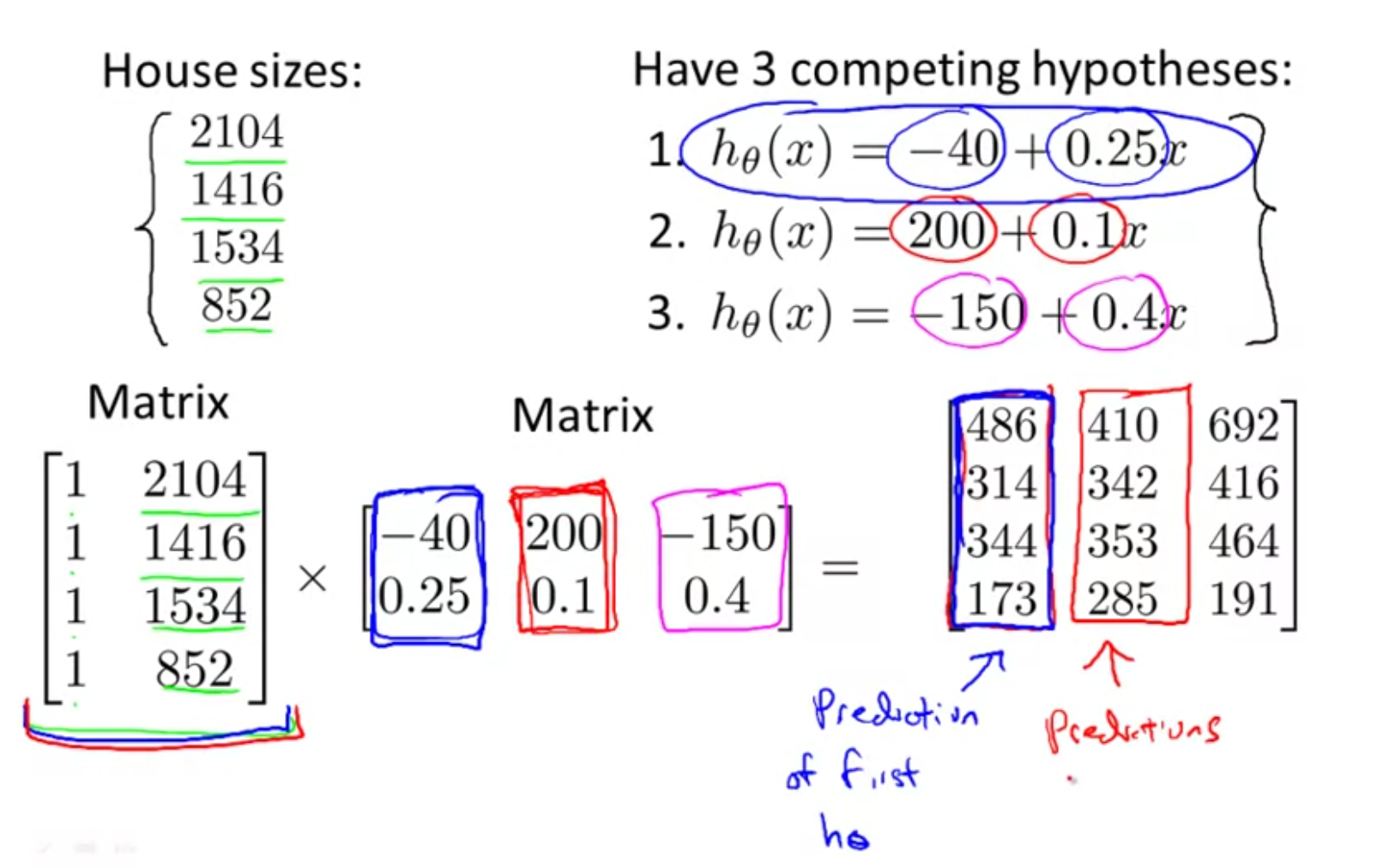
Extending the former example, suppose you want to calculate the prediction for 3 different hypothesis functions, you can represent that problem as a matrix x matrix multiplication:

Representing these as matrix operations allows programming languages to compute them in parallel, allowing for great speedups.

Properties of matrix multiplications

• Matrices are not commutative: \(A\times B \ne B\times A\)
• Matrices are associative: \((A \times B) \times C = A \times (B \times C)\)
• Identity matrix is a matrix made of ones for diagonals of same dimension such that \(A \times I = I \times A = A\)
• Identity matrix is always a square matrix.

Matrix inverse

A matrix is said to be the inverse of another matrix, if you multiply that with the matrix, you get an identity matrix. \(A \times A^{-1} = I\).

Only certain square matrices have inverses. We typically compute inverse using software.

Matrix transpose

Transpose of a matrix can be created by flipping the rows and columns. For a matrix \(A\), matrix \(B\) is said to be its transpose \(A^{T} = B\) if \(B_{ij} = A_{ji}\). In other words, \(A_{ij} = A^T_{ji}\).